16x2 LCD Module

16x2 LCD

A 16x2 LCD means it can display 16 characters per line and there are 2 such lines. In this LCD each character is displayed in 5x7 pixel matrix. This LCD has two registers, namely, Command and Data.

LCD (Liquid Crystal Display) screen is an electronic display module and find a wide range of applications. A 16x2 LCD display is very basic module and is very commonly used in various devices and circuits. These modules are preferred over seven segments and other multi segment LEDs. The reasons being: LCDs are economical; easily programmable; have no limitation of displaying special & even custom characters (unlike in seven segments), animations and so on.

The command register stores the command instructions given to the LCD. A command is an instruction given to LCD to do a predefined task like initializing it, clearing its screen, setting the cursor position, controlling display etc. The data register stores the data to be displayed on the LCD. The data is the ASCII value of the character to be displayed on the LCD. Click to learn more about internal structure of a LCD.

 

Pin Diagram: 

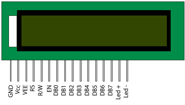
Pin No	Function	Name
1	Ground (0V)	Ground
2	Supply voltage; 5V (4.7V – 5.3V)	Vcc
3	Contrast adjustment; through a variable resistor	VEE
4	Selects command register when low; and data register when high	Register Select
5	Low to write to the register; High to read from the register	Read/write
6	Sends data to data pins when a high to low pulse is given	Enable
7	8-bit data pins	DB0
8		DB1
9		DB2
10		DB3
11		DB4
12		DB5
13		DB6
14		DB7
15	Backlight VCC (5V)	Led+
16	Backlight Ground (0V)	Led-

The LCD works with voltage pulses only and that with precise timing and voltage levels. Hence special kinds of LCD drivers are developed to drive the LCD. Two or more of this kind of driver ICs together with the LCD screen forms LCD modules which are normally found in embedded systems.The LCD module makes a system stand-alone which can take input and display the corresponding output.

Read more ...

Voltmeter

A voltmeter is an instrument used for measuring electrical potential difference between two points in an electric circuit. Analog voltmeters move a pointer across a scale in proportion to the voltage of the circuit; digital voltmeters give a numerical display of voltage by use of an analog to digital converter.
Voltmeters are made in a wide range of styles. Instruments permanently mounted in a panel are used to monitor generators or other fixed apparatus. Portable instruments, usually equipped to also measure current and resistance in the form of a multimeter, are standard test instruments used in electrical and electronics work. Any measurement that can be converted to a voltage can be displayed on a meter that is suitably calibrated; for example, pressure, temperature, flow or level in a chemical process plant.
General purpose analog voltmeters may have an accuracy of a few percent of full scale, and are used with voltages from a fraction of a volt to several thousand volts. Digital meters can be made with high accuracy, typically better than 1%. Specially calibrated test instruments have higher accuracies, with laboratory instruments capable of measuring to accuracies of a few parts per million. Meters using amplifiers can measure tiny voltages of microvolts or less.
Part of the problem of making an accurate voltmeter is that of calibration to check its accuracy. In laboratories, the Weston Cell is used as a standard voltage for precision work. Precision voltage references are available based on electronic circuits.

Analog voltmeter

A moving coil galvanometer can be used as a voltmeter by inserting a high-resistance resistor in series with the instrument. It employs a small coil of fine wire suspended in a strong magnetic field. When an electric current is applied, the galvanometer's indicator rotates and compresses a small spring. The angular rotation is proportional to the current through the coil. For use as a voltmeter, a series resistor is added so that the angular rotation becomes proportional to the applied voltage.
One of the design objectives of the instrument is to disturb the circuit as little as possible and so the instrument should draw a minimum of current to operate. This is achieved by using a sensitive galvanometer in series with a high resistance.
The sensitivity of such a meter can be expressed as "ohms per volt", the number of ohms resistance in the meter circuit divided by the full scale measured value. For example a meter with a sensitivity of 1000 ohms per volt would draw 1 milliampere at full scale voltage; if the full scale was 200 volts, the resistance at the instrument's terminals would be 200,000 ohms and at full scale the meter would draw 1 milliampere from the circuit under test. For multi-range instruments, the input resistance varies as the instrument is switched to different ranges.
Moving-coil instruments with a permanent-magnet field respond only to direct current. Measurement of AC voltage requires a rectifier in the circuit so that the coil deflects in only one direction. Moving-coil instruments are also made with the zero position in the middle of the scale instead of at one end; these are useful if the voltage reverses its polarity.
Voltmeters operating on the electrostatic principle use the mutual repulsion between two charged plates to deflect a pointer attached to a spring. Meters of this type draw negligible current but are sensitive to voltages over about 100 volts and work with either alternating or direct current.

VTVMs and FET-VMs

The sensitivity and input resistance of a voltmeter can be increased if the current required to deflect the meter pointer is supplied by an amplifier and power supply instead of by the circuit under test. The electronic amplifier between input and meter gives two benefits; a rugged moving coil instrument can be used, since its sensitivity need not be high, and the input resistance can be made high, reducing the current drawn from the circuit under test. Amplified voltmeters often have an input resistance of 1, 10, or 20 megohms which is independent of the range selected. A once-popular form of this instrument used a vacuum tube in the amplifier circuit and so was called the vacuum tube voltmeter, or VTVM. These were almost always powered by the local AC line current and so were not particularly portable. Today these circuits use a solid-state amplifier using field-effect transistors, hence FET-VM, and appear in handheld digital multimeters as well as in bench and laboratory instruments. These are now so ubiquitous that they have largely replaced non-amplified multimeters except in the least expensive price ranges.
Most VTVMs and FET-VMs handle DC voltage, AC voltage, and resistance measurements; modern FET-VMs add current measurements and often other functions as well. A specialized form of the VTVM or FET-VM is the AC voltmeter. These instruments are optimized for measuring AC voltage. They have much wider bandwidth and better sensitivity than a typical multifunction device.

Digital voltmeter

The first digital voltmeter was invented and produced by Andrew Kay of Non-Linear Systems (and later founder of Kaypro) in 1954.
Digital voltmeters (DVMs) are usually designed around a special type of analog-to-digital converter called an integrating converter. Voltmeter accuracy is affected by many factors, including temperature and supply voltage variations. To ensure that a digital voltmeter's reading is within the manufacturer's specified tolerances, they should be periodically calibrated against a voltage standard such as the Weston cell.
Digital voltmeters necessarily have input amplifiers, and, like vacuum tube voltmeters, generally have a constant input resistance of 10 megohms regardless of set measurement range.

Read more ...

Multimeter

A multimeter or a multitester, also known as a VOM (Volt-Ohm meter), is an electronic measuring instrument that combines several measurement functions in one unit. A typical multimeter would include basic features such as the ability to measure voltage, current and resistance. Analog multimeters use a microammeter whose pointer moves over a scale calibrated for all the different measurements that can be made. Digital multimeters (DMM, DVOM) display the measured value in numerals, and may also display a bar of a length proportional to the quantity being measured. Digital multimeters are now far more common than analog ones, but analog multimeters are still preferable in some cases, for example when monitoring a rapidly-varying value.
A multimeter can be a hand-held device useful for basic fault finding and field service work, or a bench instrument which can measure to a very high degree of accuracy. They can be used to troubleshoot electrical problems in a wide array of industrial and household devices such as electronic equipment, motor controls, domestic appliances, power supplies, and wiring systems.

History

The first moving-pointer current-detecting device was the galvanometer in 1820. These were used to measure resistance and voltage by using a Wheatstone bridge, and comparing the unknown quantity to a reference voltage or resistance. While useful in the lab, the devices were very slow and impractical in the field. These galvanometers were bulky and delicate.
The D'Arsonval/Weston meter movement used a fine metal spring to give proportional measurement rather than just detection, and built-in permanent field magnets made deflection independent of the orientation of the meter. Instead of balancing a bridge, values could be directly read off the instruments's scale, which made measurement quick and easy. By adding a series or shunt resistor, more than one range of voltage or current could be measured with one movement.
Multimeters were invented in the early 1920s as radio receivers and other vacuum tube electronic devices became more common. The invention of the first multimeter is attributed to British Post Office engineer, Donald Macadie, who became dissatisfied with having to carry many separate instruments required for the maintenance of the telecommunications circuits. Macadie invented an instrument which could measure amperes ( amps), volts and ohms, so the multifunctional meter was then named Avometer. The meter comprised a moving coil meter, voltage and precision resistors, and switches and sockets to select the range.
Additional scales such as decibels, and measurement functions such as capacitance, transistor gain, frequency, duty cycle, display hold, and buzzers which sound when the measured resistance is small have been included on many multimeters. While multimeters may be supplemented by more specialized equipment in a technician's toolkit, some multimeters include additional functions for specialized applications (temperature with a thermocouple probe, inductance, connectivity to a computer, speaking measured value, etc.).

Operation

A multimeter is a combination of a multirange DC voltmeter, multirange AC voltmeter, multirange ammeter, and multirange ohmmeter. An un-amplified analog multimeter combines a meter movement, range resistors and switches.
For an analog meter movement, DC voltage is measured with a series resistor connected between the meter movement and the circuit under test. A set of switches allows greater resistance to be inserted for higher voltage ranges. The product of the basic full-scale deflection current of the movement, and the sum of the series resistance and the movement's own resistance, gives the full-scale voltage of the range. As an example, a meter movement that required 1 milliampere for full scale deflection, with an internal resistance of 500 ohms, would, on a 10-volt range of the multimeter, have 9,500 ohms of series resistance.
For analog current ranges, low-resistance shunts are connected in parallel with the meter movement to divert most of the current around the coil. Again for the case of a hypothetical 1 mA, 500 ohm movement on a 1 Ampere range, the shunt resistance would be just over 0.5 ohms.
Moving coil instruments respond only to the average value of the current through them. To measure alternating current, a rectifier diode is inserted in the circuit so that the average value of current is non-zero. Since the rectified average value and the root-mean-square value of a waveform need not be the same, simple rectifier-type circuits may only be accurate for sinusoidal waveforms. Other wave shapes require a different calibration factor to relate RMS and average value. Since practical rectifiers have non-zero voltage drop, accuracy and sensitivity is poor at low values.
To measure resistance, a small battery within the instrument passes a current through the device under test and the meter coil. Since the current available depends on the state of charge of the battery, a multimeter usually has an adjustment for the ohms scale to zero it. In the usual circuit found in analog multimeters, the meter deflection is inversely proportional to the resistance; so full-scale is 0 ohms, and high resistance corresponds to smaller deflections. The ohms scale is compressed, so resolution is better at lower resistance values.
Amplified instruments simplify the design of the series and shunt resistor networks. The internal resistance of the coil is decoupled from the selection of the series and shunt range resistors; the series network becomes a voltage divider. Where AC measurements are required, the rectifier can be placed after the amplifier stage, improving precision at low range.
Digital instruments, which necessarily incorporate amplifiers, use the same principles as analog instruments for range resistors. For resistance measurements, usually a small constant current is passed through the device under test and the digital multimeter reads the resultant voltage drop; this eliminates the scale compression found in analog meters, but requires a source of significant current. An autoranging digital multimeter can automatically adjust the scaling network so that the measurement uses the full precision of the A/D converter.
In all types of multimeters, the quality of the switching elements is critical to stable and accurate measurements. Stability of the resistors is a limiting factor in the long-term accuracy and precision of the instrument.

Quantities measured

Contemporary multimeters can measure many quantities. The common ones are:

• Voltage, alternating and direct, in volts.
• Current, alternating and direct, in amperes.
  The frequency range for which AC measurements are accurate must be specified.
• Resistance in ohms.

Additionally, some multimeters measure:

• Capacitance in farads.
• Conductance in siemens.
• Decibels.
• Duty cycle as a percentage.
• Frequency in hertz.
• Inductance in henrys.
• Temperature in degrees Celsius or Fahrenheit, with an appropriate temperature test probe, often a thermocouple.

Digital multimeters may also include circuits for:

• Continuity tester; sounds when a circuit conducts
• Diodes (measuring forward drop of diode junctions), and transistors (measuring current gain and other parameters)
• Battery checking for simple 1.5 volt and 9 volt batteries. This is a current loaded voltage scale which simulates in-use voltage measurement.

Various sensors can be attached to multimeters to take measurements such as:

• Light level
• Acidity/Alkalinity(pH)
• Wind speed
• Relative humidity

Accuracy

Digital multimeters generally take measurements with accuracy superior to their analog counterparts. Standard analog multimeters measure with typically ±3% accuracy, though instruments of higher accuracy are made. Standard portable digital multimeters are specified to have an accuracy of typically 0.5% on the DC voltage ranges. Mainstream bench-top multimeters are available with specified accuracy of better than ±0.01%. Laboratory grade instruments can have accuracies of a few parts per million.
Accuracy figures need to be interpreted with care. The accuracy of an analog instrument usually refers to full-scale deflection; a measurement of 30V on the 100V scale of a 3% meter is subject to an error of 3V, 10% of the reading. Digital meters usually specify accuracy as a percentage of reading plus a percentage of full-scale value, sometimes expressed in counts rather than percentage terms.
Quoted accuracy is specified as being that of the lower millivolt (mV) DC range, and is known as the "basic DC volts accuracy" figure. Higher DC voltage ranges, current, resistance, AC and other ranges will usually have a lower accuracy than the basic DC volts figure. AC measurements only meet specified accuracy within a specified range of frequencies.
Manufacturers can provide calibration services so that new meters may be purchased with a certificate of calibration indicating the meter has been adjusted to standards traceable to, for example, the US National Institute of Standards and Technology (NIST), or other national standards organization.
Test equipment tends to drift out of calibration over time, and the specified accuracy cannot be relied upon indefinitely. For more expensive equipment, manufacturers and third parties provide calibration services so that older equipment may be recalibrated and recertified. The cost of such services is disproportionate for inexpensive equipment; however extreme accuracy is not required for most routine testing. Multimeters used for critical measurements may be part of a metrology program to assure calibration.
A multimeter can be assumed to be "average responding" to AC waveforms unless stated as being a "True RMS" type. An average responding mulimeter will only meet its specified accuracy on AC volts and amps for purely sinusoidal waveforms. A True RMS responding multimeter on the other hand will meet its specified accuracy on AC volts and current with any waveform type up to a specified crest factor.
A meter's AC voltage and current accuracy may have different specifications for different ranges of frequency.

Digital multimeters (DMM or DVOM)

Modern multimeters are often digital due to their accuracy, durability and extra features. In a digital multimeter the signal under test is converted to a voltage and an amplifier with electronically controlled gain preconditions the signal. A digital multimeter displays the quantity measured as a number, which eliminates parallax errors.
Modern digital multimeters may have an embedded computer, which provides a wealth of convenience features. Measurement enhancements available include:

• Auto-ranging, which selects the correct range for the quantity under test so that the most significant digits are shown. For example, a four-digit multimeter would automatically select an appropriate range to display 1.234 instead of 0.012, or overloading. Auto-ranging meters usually include a facility to hold the meter to a particular range, because a measurement that causes frequent range changes can be distracting to the user. Other factors being equal, an auto-ranging meter will have more circuitry than an equivalent non-auto-ranging meter, and so will be more costly, but will be more convenient to use.
• Auto-polarity for direct-current readings, shows if the applied voltage is positive (agrees with meter lead labels) or negative (opposite polarity to meter leads).
• Sample and hold, which will latch the most recent reading for examination after the instrument is removed from the circuit under test.
• Current-limited tests for voltage drop across semiconductor junctions. While not a replacement for a transistor tester, this facilitates testing diodes and a variety of transistor types.
• A graphic representation of the quantity under test, as a bar graph. This makes go/no-go testing easy, and also allows spotting of fast-moving trends.
• A low-bandwidth oscilloscope.
• Automotive circuit testers, including tests for automotive timing and dwell signals.
• Simple data acquisition features to record maximum and minimum readings over a given period, or to take a number of samples at fixed intervals.
• Integration with tweezers for surface-mount technology.
• A combined LCR meter for small-size SMD and through-hole components.

Modern meters may be interfaced with a personal computer by IrDA links, RS-232 connections, USB, or an instrument bus such as IEEE-488. The interface allows the computer to record measurements as they are made. Some DMMs can store measurements and upload them to a computer.
The first digital multimeter was manufactured in 1955 by Non Linear Systems.

Probes

A multimeter can utilize a variety of test probes to connect to the circuit or device under test. Crocodile clips, retractable hook clips, and pointed probes are the three most common attachments. Tweezer probes are used for closely spaced test points, as in surface-mount devices. The connectors are attached to flexible, thickly insulated leads that are terminated with connectors appropriate for the meter. Probes are connected to portable meters typically by shrouded or recessed banana jacks, while benchtop meters may use banana jacks or BNC connectors. 2mm plugs and binding posts have also been used at times, but are less common today.

Clamp meters clamp around a conductor carrying a current to measure without the need to connect the meter in series with the circuit, or make metallic contact at all. Types to measure AC current use the transformer principle; clamp-on meters to measure small current or direct current require more complicated sensors.

Power Supply

Analog meters can measure voltage and current using power from the test circuit but require internal power for resistance testing, electronic meters always require an internal power supply. Hand-held meters use batteries while bench meters usually use mains power allowing the meter to test devices not connected to a circuit. Such testing requires that the component be isolated from the circuit as otherwise other current paths will most likely distort measurements.

Meters intended for testing in hazardous locations or for use on blasting circuits may require use of a manufacturer-specified battery to maintain their safety rating.

Read more ...

Servo Motors mechanism

Servo Motors mechanism

A servomechanism, sometimes shortened to servo, is an automatic device that uses error-sensing negative feedback to correct the performance of a mechanism.
The term correctly applies only to systems where the feedback or error-correction signals help control mechanical position, speed or other parameters. For example, an automotive power window control is not a servomechanism, as there is no automatic feedback that controls position—the operator does this by observation. By contrast a car's cruise control uses closed loop feedback, which classifies it as a servomechanism.

Uses

Position control

A common type of servo provides position control. Servos are commonly electrical or partially electronic in nature, using an electric motor as the primary means of creating mechanical force. Other types of servos use hydraulics, pneumatics, or magnetic principles. Servos operate on the principle of negative feedback, where the control input is compared to the actual position of the mechanical system as measured by some sort of transducer at the output. Any difference between the actual and wanted values (an "error signal") is amplified (and converted) and used to drive the system in the direction necessary to reduce or eliminate the error. This procedure is one widely used application of control theory.

Speed control

Speed control via a governor is another type of servomechanism. The steam engine uses mechanical governors; another early application was to govern the speed of water wheels. Prior to World War II the constant speed propeller was developed to control engine speed for maneuvering aircraft. Fuel controls for gas turbine engines employ either hydro-mechanical or electronic governing.

Other

Positioning servomechanisms were first used in military fire-control and marine navigation equipment. Today servomechanisms are used in automatic machine tools, satellite-tracking antennas, remote control airplanes, automatic navigation systems on boats and planes, and antiaircraft-gun control systems. Other examples are fly-by-wire systems in aircraft which use servos to actuate the aircraft's control surfaces, and radio-controlled models which use RC servos for the same purpose. Many auto focus cameras also use a servomechanism to accurately move the lens, and thus adjust the focus. A modern hard disk drive has a magnetic servo system with sub-micrometre positioning accuracy. In industrial machines, servos are used to perform complex motion, in many applications.

Rotary or linear

Typical servos give a rotary (angular) output. Linear types are common as well, using a leadscrew or a linear motor to give linear motion.

Servomotor

A servomotor is a specific type of motor and rotary encoder combination, usually with a dedicated, that forms a servomechanism. This assembly may in turn form part of another servomechanism. The encoder provides position and usually speed feedback, which by the use of a PID controller allow more precise control of position and thus faster achievement of a stable position (for a given motor power).
Stepper motors are not considered as servomotors, although they too are used to construct larger servomechanisms. Stepper motors have inherent angular positioning, owing to their construction, and this is generally used in an open-loop manner, without an encoder.

Servomotors are used for both high-end and low-end applications, although the mid-range is generally handled by stepper motors. Most servomotors, at least under this name, are precision industrial components. However the very cheap radio control servo, because it combines a free-running motor and a simple position sensor with an embedded controller, also qualifies as a servomotor.

RC servos

RC servos are hobbyist remote control devices servos typically employed in radio-controlled models, where they are used to provide actuation for various mechanical systems such as the steering of a car, the control surfaces on a plane, or the rudder of a boat.
Due to their affordability, reliability, and simplicity of control by microprocessors, RC servos are often used in small-scale robotics applications.
RC servos are composed of an electric motor mechanically linked to a potentiometer. A standard RC receiver sends pulse-width modulation (PWM) signals to the servo. The electronics inside the servo translate the width of the pulse into a position. When the servo is commanded to rotate, the motor is powered until the potentiometer reaches the value corresponding to the commanded position.

   

History

James Watt's steam engine governor is generally considered the first powered feedback system. The windmill fantail is an earlier example of automatic control, but since it does not have an amplifier or gain, it is not usually considered a servomechanism.
The first feedback position control device was the ship steering engine, used to position the rudder of large ships based on the position of the ship's wheel. This technology was first used on the SS Great Eastern in 1866. Steam steering engines had the characteristics of a modern servomechanism: an input, an output, an error signal, and a means for amplifying the error signal used for negative feedback to drive the error towards zero. The Ragonnet power reverse mechanism was a general purpose air or steam-powered servo amplifier for linear motion patented in 1909.
Electrical servomechanisms were used as early as 1888 in Elisha Gray's Telautograph.

Electrical servomechanisms require a power amplifier. World War II saw the development of electrical fire-control servomechanisms, using an amplidyne as the power amplifier. Vacuum tube amplifiers were used in the UNISERVO tape drive for the UNIVAC I computer. The Royal Navy began experimenting with Remote Power Control (RPC) on HMS Champion in 1928 and began using RPC to control searchlights in the early 1930s. During WW2 RPC was used to control gun mounts and gun directors.

Modern servomechanisms use solid state power amplifiers, usually built from MOSFET or thyristor devices. Small servos may use power transistors.
The origin of the word is believed to come from the French "Le Servomoteur" or the slavemotor, first used by J. J. L. Farcot in 1868 to describe hydraulic and steam engines for use in ship steering.

The simplest kind of servos use bang–bang control. More complex control systems use proportional control, PID control, and state space control, which are studied in modern control theory.

Types of performances

Servos can be classified by means of their feedback control systems:

• type 0 servos: under steady-state conditions they produce a constant value of the output with a constant error signal;
• type 1 servos: under steady-state conditions they produce a constant value of the output with null error signal, but a constant rate of change of the reference implies a constant error in tracking the reference;
• type 2 servos: under steady-state conditions they produce a constant value of the output with null error signal. A constant rate of change of the reference implies a null error in tracking the reference. A constant rate of acceleration of the reference implies a constant error in tracking the reference.

The servo bandwidth indicates the capability of the servo to follow rapid changes in the commanded input.

Read more ...

Compact fluorescent lamp

Compact fluorescent lamp(CFL)

A compact fluorescent lamp (CFL), also called compact fluorescent light, energy-saving light, and compact fluorescent tube, is a fluorescent lamp designed to replace an incandescent lamp; some types fit into light fixtures formerly used for incandescent lamps. The lamps use a tube which is curved or folded to fit into the space of an incandescent bulb, and a compact electronic ballast in the base of the lamp.
Compared to general-service incandescent lamps giving the same amount of visible light, CFLs use one-fifth to one-third the electric power, and last eight to fifteen times longer. A CFL has a higher purchase price than an incandescent lamp, but can save over five times its purchase price in electricity costs over the lamp's lifetime. Like all fluorescent lamps, CFLs contain mercury, which complicates their disposal. In many countries, governments have established recycling schemes for CFLs and glass generally.
CFLs radiate a spectral power distribution that is different from that of incandescent lamps. Improved phosphor formulations have improved the perceived color of the light emitted by CFLs, such that some sources rate the best "soft white" CFLs as subjectively similar in color to standard incandescent lamps.

History

The parent to the modern fluorescent lamp was invented in the late 1890s by Peter Cooper Hewitt. The Cooper Hewitt lamps were used for photographic studios and industries.
Edmund Germer, Friedrich Meyer, and Hans Spanner patented a high-pressure vapor lamp in 1927. George Inman later teamed with General Electric to create a practical fluorescent lamp, sold in 1938 and patented in 1941. Circular and U-shaped lamps were devised to reduce the length of fluorescent light fixtures. The first fluorescent bulb and fixture were displayed to the general public at the 1939 New York World's Fair.
The spiral CFL was invented in 1976 by Edward E. Hammer, an engineer with General Electric, in response to the 1973 oil crisis. Although the design met its goals, it would have cost GE about $25 million to build new factories to produce the lamps, and thus the invention was shelved. The design eventually was copied by others. In 1995, helical CFLs, manufactured in China, became commercially available. Since that time, their sales have steadily increased.
In 1980, Philips introduced its model SL, which was a screw-in lamp with integral magnetic ballast. The lamp used a folded T4 tube, stable tri-color phosphors, and a mercury amalgam. This was the first successful screw-in replacement for an incandescent lamp. In 1985, Osram started selling its model EL lamp, which was the first CFL to include an electronic ballast.
Development of fluorescent lamps that could fit in the same volume as comparable incandescent lamps required the development of new, high-efficacy phosphors that could withstand more power per unit area than the phosphors used in older, larger fluorescent tubes.

Design

There are two types of CFLs: integrated and non-integrated lamps. Integrated lamps combine the tube and ballast in a single unit. These lamps allow consumers to replace incandescent lamps easily with CFLs. Integrated CFLs work well in many standard incandescent light fixtures, reducing the cost of converting to fluorescent. 3-way lamp bulbs and dimmable models with standard bases are available.
Non-integrated CFLs have the ballast permanently installed in the luminaire, and only the lamp bulb is usually changed at its end of life. Since the ballasts are placed in the light fixture, they are larger and last longer compared to the integrated ones, and they don't need to be replaced when the bulb reaches its end-of-life. Non-integrated CFL housings can be both more expensive and sophisticated. They have two types of tubes: a bi-pin tube designed for conventional ballast, and a quad-pin tube designed for an electronic ballast or a conventional ballast with an external starter. A bi-pin tube contains an integrated starter, which obviates the need for external heating pins but causes incompatibility with electronic ballasts.

Spectrum of light

CFLs emit light from a mix of phosphors inside the bulb, each emitting one band of color. Modern phosphor designs balance the emitted light color, energy efficiency, and cost. Every extra phosphor added to the coating mix improves color rendering but decreases efficiency and increases cost. Good quality consumer CFLs use three or four phosphors to achieve a "white" light with a color rendering index (CRI) of about 80, where the maximum 100 represents the appearance of colors under daylight or a black-body (depending on the correlated color temperature).
Color temperature can be indicated in kelvins or mireds (1 million divided by the color temperature in kelvins). The color temperature of a light source is the temperature of a black body that has the same chromaticity (i.e. color) of the light source. A notional temperature, the correlated color temperature, the temperature of a black body which emits light of a hue which to human color perception most closely matches the light from the lamp, is assigned.
A true color temperature is characteristic of black-body radiation; a fluorescent lamp may approximate the radiation of a black body at a given temperature, but will not have an identical spectrum. In particular, narrow bands of shorter-wavelength radiation are usually present even for lamps of low color temperature ("warm" light).
As color temperature increases, the shading of the white light changes from red to yellow to white to blue. Color names used for modern CFLs and other tri-phosphor lamps vary between manufacturers, unlike the standardized names used with older halophosphate fluorescent lamps. For example, Sylvania's Daylight CFLs have a color temperature of 3,500 K, while most other lamps called daylight have color temperatures of at least 5,000 K.

Name	Color temperature
	(K)	(Mired)
Warm/soft white	≤ 3,000	≥ 333
(Bright) white	3,500	286
Cool white	4,000	250
Daylight	≥ 5,000	≤ 200

Lifespan

CFLs typically have a rated service life of 6,000 to 15,000 hours, whereas standard incandescent lamps have a service life of 750 or 1,000 hours. However, the actual lifetime of any lamp depends on many factors, including operating voltage, manufacturing defects, exposure to voltage spikes, mechanical shock, frequency of cycling on and off, lamp orientation, and ambient operating temperature, among other factors.
The life of a CFL is significantly shorter if it is turned on and off frequently. In the case of a 5-minute on/off cycle the lifespan of some CFLs may be reduced to that of incandescent light bulbs. The U.S. Energy Star program suggests that fluorescent lamps be left on when leaving a room for less than 15 minutes to mitigate this problem. CFLs produce less light later in their lives than when they are new. The light output decay is exponential, with the fastest losses being soon after the lamp is first used. By the end of their lives, CFLs can be expected to produce 70–80% of their original light output. The response of the human eye to light is logarithmic. One photographic "f-stop" reduction represents ahalving in actual light, but is subjectively quite a small change. A 20–30% reduction over many thousands of hours represents a change of about half an f-stop. So, presuming the illumination provided by the lamp was ample at the beginning of its life, such a difference will be compensated for by the eyes.
Fluorescent lamps get dimmer over their lifetime, so what starts out as an adequate luminosity may become inadequate. In one test by the U.S. Department of Energy of "Energy Star" products in 2003–04, one quarter of tested CFLs no longer met their rated output after 40% of their rated service life.

Energy efficiency

Because the eye's sensitivity changes with the wavelength, the output of lamps is commonly measured in lumens, a measure of the power of light as perceived by the human eye. The luminous efficacy of lamps is the number of lumens produced for each watt of electrical power used. The luminous efficacy of a typical CFL is 50–70 lumens per watt (lm/W) and that of a typical incandescent lamp is 10–17 lm/W. Compared to a theoretical 100%-efficient lamp (680 lm/W), these lamps have lighting efficiency ranges of 7–10% for CFLs and 1.5–2.5% for incandescents.
Because of their higher efficacy, CFLs use between one-seventh and one-third of the power of equivalent incandescent lamps. Fifty to seventy percent of the world's total lighting market sales were incandescent in 2010. Replacing all inefficient lighting with CFLs would save 409 terawatt hours (TWh) per year, 2.5% of the world's electricity consumption. In the US, it is estimated that replacing all the incandescents would save 80 TWh yearly. Since CFLs use much less energy than incandescent lamps (ILs), a phase-out of ILs would result in less carbon dioxide (CO₂) being emitted into the atmosphere. Exchanging ILs for efficient CFLs on a global scale would achieve annual CO₂ reductions of 230 Mt (million tons), more than the combined yearly CO₂ emissions of the Netherlands and Portugal.

Failure

In addition to the wear-out failure modes common to all fluorescent lamps, the electronic ballast may fail, since it has a number of component parts. Ballast failures may be accompanied by discoloration or distortion of the ballast enclosure, odors, or smoke. The lamps are internally protected and are meant to fail safely at the end of their lives. Industry associations are working toward advising consumers of the different failure modes of CFLs compared to incandescent lamps, and to develop lamps with inoffensive failure modes. New North American technical standards aim to eliminate smoke or excess heat at the end of lamp life.

Use and adoption

CFLs are produced for both alternating current (AC) and direct current (DC) input. DC CFLs are popular for use in recreational vehicles and off-the-grid housing. There are various aid agency initiatives in developing countries to replace kerosene lamps, which have associated health and safety hazards, with CFLs powered by batteries, solar panels or wind generators.
CFLs in solar powered street lights, use solar panels mounted on the pole.
Due to the potential to reduce electric consumption and pollution, various organizations have encouraged the adoption of CFLs and other efficient lighting. Efforts range from publicity to encourage awareness, to direct handouts of CFLs to the public. Some electric utilities and local governments have subsidized CFLs or provided them free to customers as a means of reducing electric demand (and so delaying additional investments in generation).
In 2008, the European Union approved regulations progressively phasing out incandescent bulbs starting in 2009 and finishing at the end of 2012. By switching to energy saving bulbs, EU citizens will save almost 40 TW·h (almost the electricity consumption of 11 million European households), leading to a reduction of about 15 million metric tons of CO₂ emissions per year.
Australia, Canada, and the United States have also announced plans for nationwide efficiency standards that would constitute an effective ban on most current incandescent bulbs.

Venezuela and Cuba have launched massive incandescent light bulbs replacement programs in order to save energy. In the case of Venezuela, the government was able to save 2000 MW of electricity in the first six months of the 2006 program called Mission Energy Revolution, which by 2007 replaced 20 million incandescent light bulbs with CFL from a total of an estimated 55 million light bulbs in the country. Cuba replaced all the 11 million light bulbs used on the island. Also, Venezuela signed an agreement with Vietnam, one of the largest producers of CFLs in the world, to establish a factory to supply the future demand and hand-outs of government light bulbs.

Comparison
	Incandescent	Halogen	Fluorescent	LED (Generic)	LED (Philips)	LED (Philips L Prize)
Electricity usage	60 W	42 W	13 W	9 W	12.5 W	9.7 W
Lumens	860	570	660	900	800	910
Lumens/Watt	14.3	13.6	50.8	100	64	93.4
Color Temperature Kelvin	2700	3100	2700	3000	2700	2727
CRI	100	100	82	>75	85	93
Lifespan (hours)	2,000	3,500	8,000	25,000	25,000	30,000

Read more ...

Solar cell

A solar cell (also called a photovoltaic cell) is an electrical device that converts the energy of light directly into electricity by the photovoltaic effect. It is a form of photoelectric cell (in that its electrical characteristics—e.g. current, voltage, or resistance—vary when light is incident upon it) which, when exposed to light, can generate and support an electric current without being attached to any external voltage source.
The term "photovoltaic" comes from the Greek φῶς (phōs) meaning "light", and from "Volt", the unit of electro-motive force, the volt, which in turn comes from the last name of the Italian physicist Alessandro Volta, inventor of the battery (electrochemical cell). The term "photo-voltaic" has been in use in English since 1849.
Photovoltaics is the field of technology and research related to the practical application of photovoltaic cells in producing electricity from light, though it is often used specifically to refer to the generation of electricity from sunlight. Cells can be described as photovoltaic even when the light source is not necessarily sunlight (lamplight, artificial light, etc.). In such cases the cell is sometimes used as a photodetector (for example infrared detectors), detecting light or other electromagnetic radiation near the visible range, or measuring light intensity.
The operation of a photovoltaic (PV) cell requires 3 basic attributes:

1. The absorption of light, generating either electron-hole pairs or excitons.
2. The separation of charge carriers of opposite types.
3. The separate extraction of those carriers to an external circuit.

In contrast, a solar thermal collector collects heat by absorbing sunlight, for the purpose of either direct heating or indirect electrical power generation. "Photoelectrolytic cell" (photoelectrochemical cell), on the other hand, refers either a type of photovoltaic cell (like that developed by A.E. Becquerel and modern dye-sensitized solar cells) or a device that splits water directly into hydrogen and oxygen using only solar illumination.

Building block of a solar panel

Main article: Solar panel

Assemblies of photovoltaic cells are used to make solar modules which generate electrical power from sunlight. Multiple cells in an integrated group, all oriented in one plane, constitute a solar photovoltaic panel or "solar photovoltaic module," as distinguished from a "solar thermal module" or "solar hot water panel." The electrical energy generated from solar modules, referred to as solar power, is an example of solar energy. A group of connected solar modules (such as prior to installation on a pole-mounted tracker system) is called an "PV array."

History of solar cells

The photovoltaic effect was first experimentally demonstrated by French physicist A. E. Becquerel. In 1839, at age 19, experimenting in his father's laboratory, he built the world's first photovoltaic cell. Willoughby Smith first described the "Effect of Light on Selenium during the passage of an Electric Current" in an article that was published in the 20 February 1873 issue of Nature. However, it was not until 1883 that the first solid state photovoltaic cell was built, by Charles Fritts, who coated the semiconductor selenium with an extremely thin layer of gold to form the junctions. The device was only around 1% efficient. In 1888 Russian physicist Aleksandr Stoletov built the first photoelectric cell based on the outer photoelectric effect discovered by Heinrich Hertz earlier in 1887.

Albert Einstein explained the underlying mechanism of light instigated carrier excitation—the photoelectric effect—in 1905, for which he received the Nobel prize in Physics in 1921.Russell Ohl patented the modern junction semiconductor solar cell in 1946,which was discovered while working on the series of advances that would lead to the transistor.

Applications

Solar cells are often electrically connected and encapsulated as a module. Photovoltaic modules often have a sheet of glass on the front (sun up) side, allowing light to pass while protecting the semiconductor wafers from abrasion and impact due to wind-driven debris, rain, hail, etc. Solar cells are also usually connected in series in modules, creating an additive voltage. Connecting cells in parallel will yield a higher current; however, very significant problems exist with parallel connections. For example, shadow effects can shut down the weaker (less illuminated) parallel string (a number of series connected cells) causing substantial power loss and even damaging the weaker string because of the excessive reverse bias applied to the shadowed cells by their illuminated partners. Strings of series cells are usually handled independently and not connected in parallel, special paralleling circuits are the exceptions. Although modules can be interconnected to create an array with the desired peak DC voltage and loading current capacity, using independent MPPTs (maximum power point trackers) provides a better solution. In the absence of paralleling circuits, shunt diodes can be used to reduce the power loss due to shadowing in arrays with series/parallel connected cells.
To make practical use of the solar-generated energy, the electricity is most often fed into the electricity grid using inverters (grid-connected photovoltaic systems); in stand-alone systems, batteries are used to store the energy that is not needed immediately. Solar panels can be used to power or recharge portable devices.

Theory

The solar cell works in three steps:

1. Photons in sunlight hit the solar panel and are absorbed by semiconducting materials, such as silicon.
2. Electrons (negatively charged) are knocked loose from their atoms, causing an electric potential difference. Current starts flowing through the material to cancel the potential and this electricity is captured. Due to the special composition of solar cells, the electrons are only allowed to move in a single direction.
3. An array of solar cells converts solar energy into a usable amount of direct current (DC) electricity.

Efficiency

The efficiency of a solar cell may be broken down into reflectance efficiency, thermodynamic efficiency, charge carrier separation efficiency and conductive efficiency. The overall efficiency is the product of each of these individual efficiencies.
A solar cell usually has a voltage dependent efficiency curve, temperature coefficients, and shadow angles.
Due to the difficulty in measuring these parameters directly, other parameters are measured instead: thermodynamic efficiency, quantum efficiency, integrated quantum efficiency, V_OC ratio, and fill factor. Reflectance losses are a portion of the quantum efficiency under "external quantum efficiency". Recombination losses make up a portion of the quantum efficiency, V_OC ratio, and fill factor. Resistive losses are predominantly categorized under fill factor, but also make up minor portions of the quantum efficiency, V_OC ratio.
The fill factor is defined as the ratio of the actual maximum obtainable power to the product of the open circuit voltage and short circuit current. This is a key parameter in evaluating the performance of solar cells. Typical commercial solar cells have a fill factor > 0.70. Grade B cells have a fill factor usually between 0.4 to 0.7. Cells with a high fill factor have a low equivalent series resistance and a high equivalent shunt resistance, so less of the current produced by the cell is dissipated in internal losses.
Single p–n junction crystalline silicon devices are now approaching the theoretical limiting power efficiency of 33.7%, noted as the Shockley–Queisser limit in 1961. In the extreme, with an infinite number of layers, the corresponding limit is 86% using concentrated sunlight.

Cost

The cost of a solar cell is given per unit of peak electrical power. Solar-specific feed-in tariffs vary worldwide, and even state by state within various countries. Such feed-in tariffs can be highly effective in encouraging the development of solar power projects.
High-efficiency solar cells are of interest to decrease the cost of solar energy. Many of the costs of a solar power plant are proportional to the panel area or land area of the plant. A higher efficiency cell may reduce the required areas and so reduce the total plant cost, even if the cells themselves are more costly. Efficiencies of bare cells, to be useful in evaluating solar power plant economics, must be evaluated under realistic conditions. The basic parameters that need to be evaluated are the short circuit current, open circuit voltage.
The chart above illustrates the best laboratory efficiencies obtained for various materials and technologies, generally this is done on very small, i.e., one square cm, cells. Commercial efficiencies are significantly lower.
Grid parity, the point at which photovoltaic electricity is equal to or cheaper than grid power, can be reached using low cost solar cells. Proponents of solar hope to achieve grid parity first in areas with abundant sun and high costs for electricity such as in California and Japan. Some argue that grid parity has been reached in Hawaii and other islands that otherwise use diesel fuel to produce electricity. George W. Bush had set 2015 as the date for grid parity in the USA. Speaking at a conference in 2007, General Electric's Chief Engineer predicted grid parity without subsidies in sunny parts of the United States by around 2015. The Photovoltaic Association reported in 2012 that Australia has reached grid parity (ignoring feed in tariffs).
The price of solar panels fell steadily for 40 years, until 2004 when high subsidies in Germany drastically increased demand there and greatly increased the price of purified silicon (which is used in computer chips as well as solar panels). The recession of 2008 and the onset of Chinese manufacturing caused prices to resume their decline with vehemence. In the four years after January 2008 prices for solar modules in Germany dropped from €3 to €1 per peak watt. During that same times production capacity surged with an annual growth of more than 50%. China increased market share from 8% in 2008 to over 55% in the last quarter of 2010. Recently, in December 2012 the price of Chinese solar panels had dropped to $0.60/Wp (crystalline modules).

Swanson's law, an observation similar to Moore's Law that states that solar cell prices fall 20% for every doubling of industry capacity, has gained recent (as of 2012) media attention, having been featured in an article in the British weekly newspaper The Economist.

Materials

Various materials display varying efficiencies and have varying costs. Materials for efficient solar cells must have characteristics matched to the spectrum of available light. Some cells are designed to efficiently convert wavelengths of solar light that reach the Earth surface. However, some solar cells are optimized for light absorption beyond Earth's atmosphere as well. Light absorbing materials can often be used in multiple physical configurations to take advantage of different light absorption and charge separation mechanisms.
Materials presently used for photovoltaic solar cells include monocrystalline silicon, polycrystalline silicon, amorphous silicon, cadmium telluride, and copper indium selenide/sulfide.
Many currently available solar cells are made from bulk materials that are cut into wafers between 180 to 240 micrometers thick that are then processed like other semiconductors.
Other materials are made as thin-films layers, organic dyes, and organic polymers that are deposited on supporting substrates. A third group are made from nanocrystals and used as quantum dots (electron-confined nanoparticles). Silicon remains the only material that is well-researched in both bulk and thin-film forms.

Crystalline silicon

Basic structure of a silicon based solar cell and its working mechanism.

By far, the most prevalent bulk material for solar cells is crystalline silicon (abbreviated as a group as c-Si), also known as "solar grade silicon". Bulk silicon is separated into multiple categories according to crystallinity and crystal size in the resulting ingot, ribbon, or wafer.

1. monocrystalline silicon (c-Si): often made using the Czochralski process. Single-crystal wafer cells tend to be expensive, and because they are cut from cylindrical ingots, do not completely cover a square solar cell module without a substantial waste of refined silicon. Hence most c-Si panels have uncovered gaps at the four corners of the cells.
2. polycrystalline silicon, or multicrystalline silicon, (poly-Si or mc-Si): made from cast square ingots — large blocks of molten silicon carefully cooled and solidified. Poly-Si cells are less expensive to produce than single crystal silicon cells, but are less efficient. United States Department of Energy data show that there were a higher number of polycrystalline sales than monocrystalline silicon sales.
3. ribbon silicon is a type of polycrystalline silicon: it is formed by drawing flat thin films from molten silicon and results in a polycrystalline structure. These cells have lower efficiencies than poly-Si, but save on production costs due to a great reduction in silicon waste, as this approach does not require sawing from ingots.
4. mono-like-multi silicon: Developed in the 2000s and introduced commercially around 2009, mono-like-multi, or cast-mono, uses existing polycrystalline casting chambers with small "seeds" of mono material. The result is a bulk mono-like material with poly around the outsides. When sawn apart for processing, the inner sections are high-efficiency mono-like cells (but square instead of "clipped"), while the outer edges are sold off as conventional poly. The result is line that produces mono-like cells at poly-like prices.

Analysts have predicted that prices of polycrystalline silicon will drop as companies build additional polysilicon capacity quicker than the industry's projected demand. On the other hand, the cost of producing upgraded metallurgical-grade silicon, also known as UMG Si, can potentially be one-sixth that of making polysilicon.
Manufacturers of wafer-based cells have responded to high silicon prices in 2004–2008 prices with rapid reductions in silicon consumption. According to Jef Poortmans, director of IMEC's organic and solar department, current cells use between eight and nine grams of silicon per watt of power generation, with wafer thicknesses in the neighborhood of 0.200 mm. At 2008 spring's IEEE Photovoltaic Specialists' Conference (PVS'08), John Wohlgemuth, staff scientist at BP Solar, reported that his company has qualified modules based on 0.180 mm thick wafers and is testing processes for 0.16 mm wafers cut with 0.1 mm wire. IMEC's road map, presented at the organization's recent annual research review meeting, envisions use of 0.08 mm wafers by 2015.

Silicon thin films

Silicon thin-film cells are mainly deposited by chemical vapor deposition (typically plasma-enhanced, PE-CVD) from silane gas and hydrogen gas. Depending on the deposition parameters, this can yield:

1. Amorphous silicon (a-Si or a-Si:H)
2. Protocrystalline silicon or
3. Nanocrystalline silicon (nc-Si or nc-Si:H), also called microcrystalline silicon.

It has been found that protocrystalline silicon with a low volume fraction of nanocrystalline silicon is optimal for high open circuit voltage. These types of silicon present dangling and twisted bonds, which results in deep defects (energy levels in the bandgap) as well as deformation of the valence and conduction bands (band tails). The solar cells made from these materials tend to have lower energy conversion efficiency than bulk silicon, but are also less expensive to produce. The quantum efficiency of thin film solar cells is also lower due to reduced number of collected charge carriers per incident photon.
An amorphous silicon (a-Si) solar cell is made of amorphous or microcrystalline silicon and its basic electronic structure is the p-i-n junction. a-Si is attractive as a solar cell material because it is abundant and non-toxic (unlike its CdTe counterpart) and requires a low processing temperature, enabling production of devices to occur on flexible and low-cost substrates. As the amorphous structure has a higher absorption rate of light than crystalline cells, the complete light spectrum can be absorbed with a very thin layer of photo-electrically active material. A film only 1 micron thick can absorb 90% of the usable solar energy.This reduced material requirement along with current technologies being capable of large-area deposition of a-Si, the scalability of this type of cell is high. However, because it is amorphous, it has high inherent disorder and dangling bonds, making it a bad conductor for charge carriers. These dangling bonds act as recombination centers that severely reduce the carrier lifetime and pin the Fermi level so that doping the material to n- or p- type is not possible. Amorphous Silicon also suffers from the Staebler-Wronski effect, which results in the efficiency of devices utilizing amorphous silicon dropping as the cell is exposed to light. The production of a-Si thin film solar cells uses glass as a substrate and deposits a very thin layer of silicon by plasma-enhanced chemical vapor deposition (PECVD). A-Si manufacturers are working towards lower costs per watt and higher conversion efficiency with continuous research and development on Multijunction solar cells for solar panels. Anwell Technologies Limited recently announced its target for multi-substrate-multi-chamber PECVD, to lower the cost to US$0.5 per watt.

Amorphous silicon has a higher bandgap (1.7 eV) than crystalline silicon (c-Si) (1.1 eV), which means it absorbs the visible part of the solar spectrum more strongly than the infraredportion of the spectrum. As nc-Si has about the same bandgap as c-Si, the nc-Si and a-Si can advantageously be combined in thin layers, creating a layered cell called a tandem cell. The top cell in a-Si absorbs the visible light and leaves the infrared part of the spectrum for the bottom cell in nc-Si.

Manufacture

Because solar cells are semiconductor devices, they share some of the same processing and manufacturing techniques as other semiconductor devices such as computer and memory chips. However, the stringent requirements for cleanliness and quality control of semiconductor fabrication are more relaxed for solar cells. Most large-scale commercial solar cell factories today make screen printed poly-crystalline or single crystalline silicon solar cells.
Poly-crystalline silicon wafers are made by wire-sawing block-cast silicon ingots into very thin (180 to 350 micrometer) slices or wafers. The wafers are usually lightly p-type doped. To make a solar cell from the wafer, a surface diffusion of n-type dopants is performed on the front side of the wafer. This forms a p–n junction a few hundred nanometers below the surface.
Anti-reflection coatings, to increase the amount of light coupled into the solar cell, are typically next applied. Silicon nitride has gradually replaced titanium dioxide as the anti-reflection coating, because of its excellent surface passivation qualities. It prevents carrier recombination at the surface of the solar cell. It is typically applied in a layer several hundred nanometers thick using plasma-enhanced chemical vapor deposition (PECVD). Some solar cells have textured front surfaces that, like anti-reflection coatings, serve to increase the amount of light coupled into the cell. Such surfaces can usually only be formed on single-crystal silicon, though in recent years methods of forming them on multicrystalline silicon have been developed.
The wafer then has a full area metal contact made on the back surface, and a grid-like metal contact made up of fine "fingers" and larger "bus bars" are screen-printed onto the front surface using a silver paste. The rear contact is also formed by screen-printing a metal paste, typically aluminium. Usually this contact covers the entire rear side of the cell, though in some cell designs it is printed in a grid pattern. The paste is then fired at several hundred degrees Celsius to form metal electrodes in ohmic contact with the silicon. Some companies use an additional electro-plating step to increase the cell efficiency. After the metal contacts are made, the solar cells are interconnected by flat wires or metal ribbons, and assembled into modules or "solar panels". Solar panels have a sheet of tempered glass on the front, and a polymer encapsulation on the back.

Lifespan

Most commercially available solar panels are capable of producing electricity for at least twenty years. The typical warranty given by panel manufacturers is over 90% of rated output for the first 10 years, and over 80% for the second 10 years. Panels are expected to function for a period of 30 to 35 years.

Read more ...